Calculators, Power Series and Chebyshev Polynomials: Unterschied zwischen den Versionen
(→Conclusion --- The point of the story) |
|||
| Zeile 222: | Zeile 222: | ||
The procedure above is called ''economization of power series''. As mentioned in the Introduction, there are other methods of | The procedure above is called ''economization of power series''. As mentioned in the Introduction, there are other methods of | ||
speeding up the calculation of values of the trigonometric functions, such as the Cordic algorithm for the sine function, but | speeding up the calculation of values of the trigonometric functions, such as the Cordic algorithm for the sine function, but | ||
| − | economization is considered to be essential for ''slowly converging'' series such as that for <math\tan^{-1}x\,</math> | + | economization is considered to be essential for ''slowly converging'' series such as that for <math>\tan^{-1}x\,</math> |
established in (3), above. Perhaps the point of this story is that, very often, the obvious approach is not necessarily best. | established in (3), above. Perhaps the point of this story is that, very often, the obvious approach is not necessarily best. | ||
Version vom 28. Juni 2010, 09:27 Uhr
Originating author: Graeme Cohen
Inhaltsverzeichnis |
Introduction --- Functions on a calculator
Of all the familiar functions, such as trigonometric, exponential and logarithmic functions, surely the simplest to evaluate are
polynomial functions. One purpose of this note is to introduce the concept of a power series, which can be thought of in the
first place as a polynomial function of infinite degree. In particular, we will deduce a series for  and
will see how to improve on the the most straightforward way of approximating its values. This simplest way uses the polynomials
obtained by truncating the power series. The improvement will involve Chebyshev polynomials, which are used in many ways for
a similar purpose and in many other applications, as well. When a calculator gives values of trigonometric or exponential or
logarithmic functions it is doing so by evaluating polynomial functions that are sufficiently good approximations. So we have the
second purpose of this note: the realization that although the mathematics here would have been known to Felix Klein at the
beginning of the 20th century, new applications are always arising and the one described here, to finding values of functions on
a calculator, would clearly not have been known to him. (We point out that, for trigonometric functions, the CORDIC algorithm
is in fact often the preferred method of evaluation---the subject of another article here, perhaps.)
and
will see how to improve on the the most straightforward way of approximating its values. This simplest way uses the polynomials
obtained by truncating the power series. The improvement will involve Chebyshev polynomials, which are used in many ways for
a similar purpose and in many other applications, as well. When a calculator gives values of trigonometric or exponential or
logarithmic functions it is doing so by evaluating polynomial functions that are sufficiently good approximations. So we have the
second purpose of this note: the realization that although the mathematics here would have been known to Felix Klein at the
beginning of the 20th century, new applications are always arising and the one described here, to finding values of functions on
a calculator, would clearly not have been known to him. (We point out that, for trigonometric functions, the CORDIC algorithm
is in fact often the preferred method of evaluation---the subject of another article here, perhaps.)
In the spirit of Felix Klein, there will be some reliance on a graphical approach.
Manipulations with geometric series
The geometric series  is the simplest power series. The sum of the series exists when
 . In fact,

The general form of a power series is

so the geometric series above is a power series in which all the coefficients  ,
,  ,
,
 ,
,  , are equal to 1. In this case, since the series converges to
  when
, we say that the function
when
, we say that the function  , where
has the series expansion , or that is represented by this series. We are
interested initially to show some other functions that can be represented by power series.
Many such functions may be obtained directly from the result in (1). For example, by replacing  by
by
 , we immediately have a series representation for the function
  :
:

We can differentiate both sides of (1) to give a series representation of the function  :
:
We can also integrate both sides of (1). Multiply through by  (for convenience), then write
  for
and integrate with respect to from 0 to , where :
for
and integrate with respect to from 0 to , where :
so

So this gives a series representation of the function  , . In the same way, from (2),

Much of what we have done here (and will do later) requires justification, but we can leave that to the textbooks.
A series for the sine function
We will show next how to find a power series representation for the sine function.
In general terms, we can write

Put  , and immediately we have
  . Differentiate both sides of (4):

Again put , giving  . Keep differentiating and putting :

so  ,
,

so 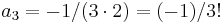 ,
,

so  ,
,

so 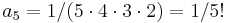 .
.
In this way, we can find a formula for all the coefficients , , ,
, namely,

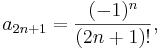
for  , 1, 2, . (The coefficients of even index and those of odd index are specified
separately.)
, 1, 2, . (The coefficients of even index and those of odd index are specified
separately.)
Thus
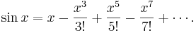
This is the power series representation that we were after.
Using Chebyshev polynomials
From the way we developed it, it is reasonable that this series will represent for values of
at and near 0 (say for , as for all the earlier examples), so it is surprising to know that it
can be shown that the series represents for all values of . Then partial sums of the
series, obtained by stopping after some finite number of terms, should give polynomial functions that can be used to find
approximate values of the sine function, such as you find in tables of trigonometric functions or as output on a calculator.
For example, write
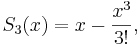
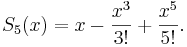
The cubic polynomial  and the quintic polynomial
  are plotted below, along with , all for
  . It can be seen that these are both very good approximations for
  , say, but not so good near
  . The quintic
  is much better than the cubic
 in these regions, as might be expected, but can we do better than with some other cubic
polynomial function?
in these regions, as might be expected, but can we do better than with some other cubic
polynomial function?
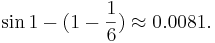
When  , for example, the error in using the cubic is
We will construct a cubic polynomial function  whose values differ from those of by less
than 0.001 for
whose values differ from those of by less
than 0.001 for  . The curve
  has been included in the graph below for
  ,
and it is clear from the graph that this curve is closer to that of
,
and it is clear from the graph that this curve is closer to that of  than
than  is, even
near .
is, even
near .
We will use Chebyshev polynomials to construct . These are used extensively in approximation problems, as we
are doing here. They are the functions  given by

for integer  . By properties of the cosine, they all have domain
 ![[-1,1]](/images/math/d/0/6/d060b17b29e0dae91a1cac23ea62281a.png) and their range is also in
. Putting
and their range is also in
. Putting  and
and  gives
gives
but it is not immediately apparent that the are indeed polynomials for  . To see that this is
the case, recall that
. To see that this is
the case, recall that


from which, after adding these,

Therefore,

Now put  and obtain


and so on, clearly obtaining a polynomial each time. As polynomials, we no longer need to think of their domains as restricted to
.
Returning to our problem of approximating for with error less than 0.001, we notice
first that the quintic has that property. In fact,

and the theory of alternating infinite series shows that 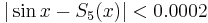 throughout our interval, as
certainly seems reasonable from the figure. We next express in terms of Chebyshev polynomials. Using (5) and
(6), we have
throughout our interval, as
certainly seems reasonable from the figure. We next express in terms of Chebyshev polynomials. Using (5) and
(6), we have

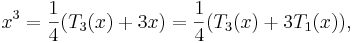

so

Since  when , omitting the term
  will admit a
further error of at most
will admit a
further error of at most 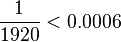 which, using (7), gives a total error less than 0.0008, still within
our bound of 0.001. Now,
which, using (7), gives a total error less than 0.0008, still within
our bound of 0.001. Now,

and the cubic function we end with is the function we called .
We have thus shown, partly through a graphical justification, that values of the cubic function , where
are closer to values of , for , than are values of the cubic function
 , which is obtained from the power series representation of .
Conclusion --- The point of the story
The effectiveness of Chebyshev polynomials for such a purpose arises from properties of the cosine function. They tell us in
particular that for all integers and for , we have  . Pafnuty
Lvovich Chebyshev was Russian; he introduced these polynomials in a paper in 1854. His surname is often given alternatively as
Tchebycheff, and this is why the polynomials are denoted with <mathT\,<\math>'s.
. Pafnuty
Lvovich Chebyshev was Russian; he introduced these polynomials in a paper in 1854. His surname is often given alternatively as
Tchebycheff, and this is why the polynomials are denoted with <mathT\,<\math>'s.
The procedure above is called economization of power series. As mentioned in the Introduction, there are other methods of
speeding up the calculation of values of the trigonometric functions, such as the Cordic algorithm for the sine function, but
economization is considered to be essential for slowly converging series such as that for  established in (3), above. Perhaps the point of this story is that, very often, the obvious approach is not necessarily best.