Higher Dimensions: Unterschied zwischen den Versionen

Version vom 8. Februar 2012, 20:26 Uhr

Inhaltsverzeichnis

1 Looking for the next dimension
2 Geometry of coordinates
3 Projections
4 Intersections of cubes
5 Quasicrystals – Projections from higher dimensions
6 Conclusion
7 References

Looking for the next dimension

Fig. 1: Illustration of a Calabi-Yau-manifold (Important for the description of higher dimensional models in superstring-theory)

Does our world really have more than three dimensions? If so, do objects in higher dimension have a relation to the world around us? Is it possible to get a perception of these objects or do they withdraw any representation? Questions like these will be posed by students if you talk about space dimensions in school. Students want to understand the meaning of a four-, five or even n-dimensional space. The relativity theory uses four dimensions to explain the concept of space-time, six dimensions are necessary to describe the bending of space-time and different string theories even use representations in up to 26 dimensions (e.g. L. Botelho, R. Botelho, 1999). Another current domain of application for higher dimensional objects and their three-dimensional representations is the study of non-periodic structures in modern crystallography. Within the concept of quasicrystals projections of higher dimensional point-sets (such as the integer-lattice in dimension 5) to three dimensional space are supposed to be good models for non-periodic crystalline structures (see section 5 below).

These examples show one of the main characteristics of mathematical thinking: If it is easier or helpful to describe real phenomena in higher dimensional space, the three special dimensions can be extended. This can easily be explained under formal aspects. Thus, linear equations with three variables may be interpreted as a plane in space, linear equations with four variables are interpreted as a three dimensional hyper plane in a four dimensional space. Also, linear equations with n-variables are interpreted as an (n-1)-dimensional hyper plane in an n-dimensional space. While using more than three variables, the advantage of such an expansion of the dimension-concept benefits from a simpler and more consistent description of mathematical relations. It is not necessary for formal calculations on an algebraic and numerical level to have illustrative perceptions in such a higher dimensional context. Nevertheless, on the one hand this leads to the question how to translate the results of such considerations into the real world. On the other hand there is a need to describe at least basic objects of higher dimensions in our three dimensional space.

In the following, thoughts dealing with the development of representations of higher dimensional objects will be discussed by exemplarily considering a four-dimensional object, the four-dimensional cube. It will be shown that the approach to four- and higher-dimensional cubes can be done in different ways. The extensive use of analogical considerations serves as a basis for understanding higher dimensional objects. In the following, three different approaches will be shown and analyzed (A detailed description of these approaches is found in Ruppert (2010)).

(1) A systematic extension of the concept of coordinates,
(2) Projections of higher-dimensional objects on (hyper)planes,
(3) Intersections of (hyper)cubes and a (hyper)plane.

Geometry of coordinates

The unit line segment and the unit square can be considered as a one‐ or two‐dimensional analog of the unit cube. Looking at the coordinates of the vertices in a coordinate system, we get

Vertices of the unit line-segment:	$A_{1}= (0)$	$A_{2}= (1)$
Vertices of the unit square:	$A_{1}= (0 \mid 0)$	$A_{2}= (1 \mid 0)$	$A_{3}= (0 \mid 1)$	$A_{4}= (1 \mid 1)$
Vertices of the unit cube:	$A_{1}= (0 \mid 0 \mid 0)$	$A_{2}= (1 \mid 0 \mid 0)$	$A_{3}= (0 \mid 1 \mid 0)$	$A_{4}= (1 \mid 1 \mid 0)$
	$A_{5}= (0 \mid 0 \mid 1)$	$A_{6}= (1 \mid 0 \mid 1)$	$A_{7}= (0 \mid 1 \mid 1)$	$A_{8}= (1 \mid 1 \mid 1)$

By successively adding additional coordinates with coefficients 0 and 1, the coordinates of the vertices and thus the number of vertices of a unit hyper cube in a four‐ or five‐dimensional coordinate system are obtained. The transition to hyper cubes in higher dimensions can exclusively be accomplished on a symbolical level and can be considered as a continuation of the concept of the coordinates. Combinatorial considerations lead to the following relation for the number N(n;k) of the k‐dimensional “boundary cubes” of an n‐dimensional cube (see e. g. Graumann, 2009):

$N(n;k)={n \choose k} \cdot 2^{n-k}$

This formula can be obtained by the following observations:

Every k‐dimensional “boundary‐cube” is parallel to a k‐dimensional hyperplane which is spanned by k generating vectors of the n‐dimensional cube (see also sec. 3). As a consequence, the coordinates of vertices belonging to one and the same k‐dimensional “boundary‐cube” differ in at most k coefficients (and all such vertices belong to this cube).
There are ${n \choose k}$ possibilities to choose k coefficients out of n.
There are 2ⁿ possibilities to choose a "starting vertex".
There are 2^k starting vertices leading to the same boundary cube.

Example 1: The three‐dimensional cube (n = 3):

Table 1: Number of the k‐dimensional boundaries of an n‐dimensional cube

Number of vertices (k= 0):	$N(3;0)={3 \choose 0} \cdot 2^{3-0} = 8$
Number of edges (k= 1):	$N(3;1)={3 \choose 1} \cdot 2^{3-1} = 12$
Number of faces (k= 2):	$N(3;2)={3 \choose 2} \cdot 2^{3-2} = 6$
Number of cubes (k= 3):	$N(3;3)={3 \choose 3} \cdot 2^{3-3} = 1$

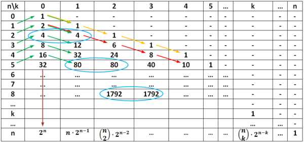
This can be illustrated in table 1.
First of all, following the yellow highlights, the table allows the interpretation of a single point as a cube of dimension 0, so that the formula above is consistent even for n = 0. The number sequences highlighted in different colors lead to further conjectures, which can be proved by using the formula for N(n;k) above. For instance:

$N(n;n-1)=2n$ (red color)

$n \cdot N(n-1;0)=N(n;1)$ (green color)

$For\ all\ t\ge 1:\ N(3t-1;t-1) = N(3t-1;t)$ (blue color)

Moreover, a recursive formula is given, to calculate the data of the n‐dimensional cube of the corresponding numbers for the (n-1)‐dimensional cube

$N(n;k)= 2 \cdot N(n-1;k) + N(n-1;k-1)$ .

Example 2: Proof of the recursive formula

$N(n;k)= 2 \cdot N(n-1;k) + N(n-1;k-1)$	$=$	$2 \cdot {n-1 \choose k} \cdot 2^{n-1-k} + {n-1 \choose k-1} \cdot 2^{n-1-(k-1)}$
	$=$	$\left[{n-1 \choose k}+{n-1 \choose k-1} \right] \cdot 2^{(n-k)}$
	$=$	$N(n;k)={n \choose k} \cdot 2^{n-k}$
	$=$	$N(n;k)$

Of course, these algebraic arguments can easily be reinterpreted geometrically and retransformed to the geometric situation.

Projections

In the following, the basic idea of describing higher dimensional objects by means of projection will be generalized in higher dimensions. Especially the orthogonal projection along a body diagonal of an n-dimensional hyper cube (i.e. the line segment from (0, . . . , 0) to (1, . . ., 1)) in an (n-1)-dimensional space can easily be generalized.

Example 3: Projections of square and cube

//

Bei der MediaWiki-Programmerweiterung GeoGebra ist ein Fehler aufgetreten: Ein Parameter wurde nicht angegeben und fehlt daher („width“, „height“ oder „ggbBase64“).

Fig. 2.1: Projection of a square (Author: Sebastian Hammer, University of Würzburg)

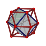
Fig. 2.2:Projection of a cube (Author: Sebastian Hammer, University of Würzburg)

Fig. 3.1: Projection of a 4D-hyper cube; Eight of the projected edges point to the vertices of a 3D-cube

Fig. 3.2: Projection of a 4D-hyper cube; virtuel model

For $1\le i \le 4$ let A_i (Sec. 2) be the vertices of the square. The projection of Fig. 2.1 is represented by the intersection of the straight lines

$g_{i}: \ \vec{X}= \vec{A_{i}} + k \cdot \begin{pmatrix}1 \\ 1 \end{pmatrix} , \ \ (1\le i \le 4)$ with the line $h:\ x_{1}+x_{2}=0.$

This is an orthogonal projection. Similarly, the orthogonal projection of an n-dimensional hyper cube is fully described by the projection of the coordinates of the vertices $A_{i}(1\le i \le 2^{n})$ . We look for the intersection points of the straight lines:

$g_{i}: \ \vec{X}= \vec{A_{i}} + k \cdot \begin{pmatrix}1 \\ \vdots \\1 \end{pmatrix} , \ \ (1\le i \le 2^{n})$ and the (n-1)-hyper-plane $R:\ x_{1}+ \cdots +x_{2}=0.$

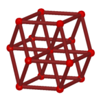
The vector $(1,1,...,1)$ is orthogonal to the hyperplane R, the lines g_i are the orthogonal lines to the hyperplane R through the vertices A_i. After considering similarities of the projections above, such as vertices having the same image under these special mappings, we get Fig. 3.2 as representation for the corresponding orthogonal projection of a four-dimensional hyper cube into the three-dimensional space.

Another possibility to describe orthogonal projections from n-dimensional into k-dimensional space $(k \le n)$ uses the linearity of orthogonal projections (as linear transformations). This property can be used to create and understand two-dimensional images of cubes of any dimension.

Example 4: Projection of a cube

Fig. 4.1: A projection of the five-dimensional unit cube on a plane

Fig. 4.2: A projection of the six-dimensional unit cube on a plane

Fig. 2 shows three generating vectors of the cube and their images under orthogonal projection along the body-diagonal. All vertices of the cube are linear combinations of these vectors with coefficients 0 and 1. The linearity of the projection leads to the same property for the images of all vertices.

While describing the n-dimensional cube with adequate linear combinations of n linear independent generating vectors, the following can be shown: For the n-dimensional cube, there is an orthogonal projection into R² and an appropriate plane of projection, such that the images of the generating vectors point to the vertices of a regular n-sided polygon. According to additivity, the images of all the other vertices finally result in corresponding linear combinations. (For n=3 see Fig. 2 and Example 3, with the regular triangle as image of the generating vectors)

To understand how the projection of an n-dimensional hypercube on a k-dimensional subspace is obtained we first explain how a cube is projected onto a line in the three-dimensional space:
For each vertex of the cube take the plane orthogonal to the given line which contains this vertex. The intersection point of the plane and the line is the orthogonal projection of the vertex onto the line.

Analogously we project the n-dimensional hypercube on a k-dimensional plane. For each vertex of the hypercube take the (n-k)-dimensional plane orthogonal to the given k-dimensional plane which contains this vertex. The intersection point of these two hyperplanes is the orthogonal projection of the vertex onto the k-dimensional subspace.

So, a two-dimensional projection of the five-dimensional unit cube can be indicated: Based on the images of the generating vectors (pointing to the vertices of a regular pentagon), the images of any vertices can be found by appropriately adding those vectors.

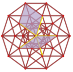
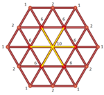
Looking at the projection of the five-dimensional cube, the images of the edges of the cubes span the well-known Penrose-Rhombs (see Senechal 1995). Another remarkable phenomenon is shown in figure 4.2. Under the projection of the six-dimensional Hypercube along its body-diagonal – the line segment with the endpoints $(0, 0, 0, 0, 0, 0)$ to $(1, 1, 1, 1, 1, 1)$ – there are several vertices with the same projection. The number of preimages is also given in Fig. 4.2.

Intersections of cubes

A dynamic representation of a four-dimensional hypercube is given by considering the different shapes of intersection while intersecting it with a three-dimensional hyper plane. Initially, a cube (in a three-dimensional space), which interacts a plane will be regarded. It is assumed, that the objects move with (relative) velocity v. It is especially easy to describe the situation while considering the cube (edge length a) with its edges fixed on the axes of a coordinate system. The plane $E(t):\ x_{1}+x_{2}+x_{3}-\sqrt{3} \cdot v \cdot t = 0$ moves along a cube diagonal with velocity v through this cube. Since the cube is a convex body itself, it is sufficient to determine the points of intersection of the edges at any time. We get the cross section as the convex hull of these intersection points. In the following, shapes of intersection will be shown in chronological order:

The intersection of a three-dimensional space while moving through a four-dimensional hypercube will be analogously represented as follows:

A four-dimensional hypercube with an edge length $a$ will be intersected with a space $R(t)$ , which moves with a velocity of $v$ along the body diagonal of the hypercube. Therefore we define analogously: $R(t):\ x_{1}+x_{2}+x_{3}+x_{4}-2 \cdot v \cdot t = 0$ .

Again, it is sufficient to know the intersection points of the hypercube with R. As a convex hull of these intersection points, we get the following shapes of intersection, which are shown in chronological order:

An interactive simulation of these intersections in one to four dimensions is given in the following applet (Author: Rafael Losada, Instituto GeoGebra de Cantabria).

Quasicrystals – Projections from higher dimensions

Starting with the assumption of the classical crystallography, that the characteristic of real crystallographic structures is their translational symmetry (i.e. invariance under three independent translations), mathematical representations of these structures lead to the well-known “crystallographic restriction”, which allows non-trivial rotational symmetries only of orders 2, 3, 4 and 6. This corresponds to physical observations, until Shechtman et al. (1984) found a non-periodic structure of crystals (without translational symmetry) inside an Al-Mn-alloy, which has fivefold rotational symmetry. Christallographers call these structures quasicrystals. To be more precise:

Quasicrystals are structural forms that are ordered but not periodic. They form patterns that fill all the space though they lack translational symmetries.

But these quasicrystals can be very complicated: the lack of translational symmetries leads to a lack of rules to explain how the pattern develops far from a region we are observing. This represents a challenge for the mathematician to explain the pattern. A breakthrough has occurred by the observation that many quasicrystals that look aperiodic are simply projections on a lower dimensional affine subspace of a regular grid in a higher dimensional space. Indeed, let us look at a simple example...

Fig. 5: One-dimensional quasicrystal

Example 5: One-dimensional quasicrystals

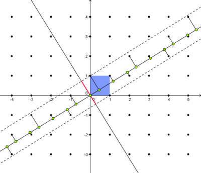
For the line $g_{1}:\ y=(\tau -1) \cdot x$ in R² and its orthogonal $g_{2}:\ y= {\frac{1}{1 - \tau}} \cdot x$ line through the origin with $\tau= \frac {1}{2} + \frac {1}{2} \sqrt{5}$ we consider the orthogonal projection of the unit square on g₂ (red line segment). Further we look at all points of Z⁵ with images under this projection lying on the red line segment. These points are now projected orthogonally on g₁ (green points).

The length of the line segments on the projection line can take only two values (corresponding to the projection of the edges of the unit square). Thus we can speak of an “ordered structure”. Moving along the lines, the sequence of these values looks more or less chaotic - there is no translational symmetry, but if we enlarge the universe to two dimensions, then everything becomes clear: our quasicrystal is just the projection of a regular square grid. Enlarging the dimension has allowed us to understand the hidden structure of the quasicrystal.
This process is quite general. Senechal (1995) for instance illustrates regularities and assumptions for projection methods and multigrid methods which lead to quasi-crystalline point-sets. Projecting, for example, parts of a five-dimensional cubic grid (Z⁵) to a certain plane, a point-set, like in the above sense, is obtained and can be regarded as a two-dimensional quasicrystal. The point-set itself shows all vertices of the Penrose-tiling of the plane (by the two characteristic rhombs, compare section 3 and image 2).

Conclusion

We have discovered one way how the mathematician works, which is sometimes summarized by the following sentence

"Mathematics makes the invisible visible"

When you don’t understand something, you try to change your point of view. It may happen that the new point of view gives an explanation of the hidden structure. This is already what you do when you try to understand a conic: you choose an appropriate system of coordinates in which the equation is simple and reveals the features of the conic.

The benefits students will get out of the working with objects in higher dimensions are manifold. They will especially

get a first insight into the meaning of higher dimensions in science;
get to know different possibilities of an access to objects in higher dimensions;
use analogies to extend their knowledge of the well‐known three dimensional world and they will use the properties of the objects in this world as an abstract concept of a mental fictive world;
refresh and repeat their knowledge about projections of three dimensional objects in a plane.

References

BOTELHO, L.; BOTELHO, R.: Quantum Geometry of bosonic strings – Revisited. Notas de Física, Centro Brasileira de Pesquisas Físicas (1999).
CAYLEY, A.: On Jacobi's elliptic functions, in reply to the Rev..; and on quaternions. Philosophical Magazine. (1845) Nr. 26, S. 208–211.
DELONE B.N., Geometry of positive quadratic forms, Usp. Mat. Nauk 3 (1937), S. 16‐62, und Usp. Mat. Nauk 4 (1938), S. 102‐164. (Russisch)
GRAUMANN, G.: Spate in drei und mehr Dimensionen. MU 55/1 (2009), S. 16‐25
HAMILTON, W. R.: On quaternions, or an new system of imagineries in algebra. Philosophical Magazine.(1844) Bd. 25(3), S. 489‐495.
LAGARIAS, J.: Meyer’s concept of quasicrystal and quasiregular sets. Community of Mathematical Physics 179 (1996), S. 365‐376.
MEYER, Y.: Algebraic numbers and harmonic analysis. North Holland (1972)
RIEMANN, B.: Ueber die Darstellbarkeit einer Function durch eine trigonometrische Reihe (Habil.). Abhandlungen der Königlichen Gesellschaft der Wissenschaften zu Göttingen, Bd. 13 (1868)
RUPPERT, M.: Würfelbetrachtungen. Drei Wege zu höheren Dimensionen. MU 56/1 (2010), S. 34‐53.
SCHLÄFLI, L.: Theorie der vielfachen Kontinuität (1852). Denkschrift der Schweizerischen Naturforschenden Gesellschaft, Bd. 38, 1., Hrsg. Graf, J. H. (1901), S. 1‐237.
SENECHAL, M.: Quasicrystals and geometry. Cambridge University Press (1995)

The development of the concept of higher dimensional geometry was started with Hamilton’s (1844), Cayley’s (1845), Schläfli’s and Riemann’s scientific works.

@@ Zeile 143: / Zeile 143: @@
 <br/>
-<ggb_applet width="810" height="570"  version="4.0" ggbBase64="UEsDBBQACAAIAJR5REAAAAAAAAAAAAAAAAAWAAAAZ2VvZ2VicmFfamF2YXNjcmlwdC5qc0srzUsuyczPU0hPT/LP88zLLNHQVKiu5QIAUEsHCEXM3l0aAAAAGAAAAFBLAwQUAAgACACUeURAAAAAAAAAAAAAAAAADAAAAGdlb2dlYnJhLnhtbOVc63LbNhb+3T4FRj8yyU5lESB4S+V2ZDnZZpo22Trb2dk/OxAJSYwpUiEpW8r0AfZN9r32SfYAIGlSNGXRklzJ67FNEQBxOd93Ljgk1f9xOQvQDY8TPwrPO/hM6yAeupHnh5PzziIdd+3Ojz9825/waMJHMUPjKJ6x9LxDRUvfO++Y+piOqed2x4amdenINLuOicddy8QE22OGucs7CC0T/3UY/cpmPJkzl1+5Uz5j7yOXpXLgaZrOX/d6t7e3Z/lQZ1E86U0mo7Nl4nUQTDNMzjvZh9fQXeWiW102J5qGe//45b3qvuuHScpCMb5YwsL/4dtv+rd+6EW36Nb30iksmFJYx5T7kyksyjbMDuqJVnOQyJy7qX/DE7i2dCoXnc7mHdmMhaL+G/UJBcV6Osjzb3yPx+cd7QxjHTu09NNBUezzMM0a42zQXt5d/8bnt6pf8UkOCRelURSMmOgS/fEHIhrR0HfigNWBwME0VZWmyjRdHYg6UHUwVBuqLqeqKVVtqGpD9Q668RN/FPDzzpgFCcjQD8cx4FecJ+kq4HI+WcHd8vF3sKbE/wqNdQ0ErIQO5Zr2nfgz4Y+Kil51kbg0ahovWg6aD4mpTrYfk+y0Ur0Y1NTrYxKjYZ3mhkHVwrdaqFGSLQwlf+VfbUR90zLXR1Tnuw1o0idZYr+X60o/Uw+UTEXbjD4pnyVCYXQHGY7gPUYGKIdpAc0NhB04WASBOiBsIGrAKbaRKY4W0i2ooEhHNhLtsI6kdhg2/KOW7MxEBnQmSi1QSoRhIIoMHWGpVBSBKiGpmKCkRIcWhoEMuEgMj4noQjcRNeFMtxGFOQqdtDA01OFCOIfhCdIx0sXF2ELERKboD1Oh66Ytpg5dEmRqyMSiQ1BrUGmlztDeRrpYTW7Y/HC+SCsicmde/jGN5gUW0BoM0p3dUwaqYha/6QdsxANwFVcCSYRuWCA0Qg40jsIU5SASVTaJ2Xzqu8kVT1O4KkGf2Q17z1K+fAutk3xs2daNwuRjHKXDKFjMwgQhNwq0Ys5RgEufSTFrONFLFbRcYZQqzNJn695xI6hBi4TD+FGc5M2Z570TLe5MA0jyQxisLmLOrueRX11Gvye9Tp8v3MD3fBb+DmQVowi5oDsnJLQzd0IWUDubSRR7V6sEKIyW/+RxBLaKaGcaNsCkOOC5TFMDWFeqimrWmaUTalDLJrZmC8PkMqF8FgYPhClcopuWozugmKv7q2ysRuY3BUJsye8WO4mFZpdO3iUXUXBXJNc/ZPN0Ecv4AeYQi0UNwknAJUekuQXn7F6PouWVIoeu+vq0msNZtvbRRModgW0AZwQNsuNIHWUbMbWilSbbaLKFlrPN94p67BDZQh5H6ihbAX3V1LKl4nyZWMuH8RNp0bROpje5tRLkF65+Efrp+/wk9d3rbKlYXfDrYjbiBYWqfeJ99dnvrXGsf83jkAcZpQHMRbRIlIaW2O5x15/BqarIRMIEXH+HCahSj09ink88kLGZEpisrZC1Viy7ehtHs3fhzSfgwtoE+r18lv3Ejf254BwagRu45nes8vyEgRfxytcJHYSlu8JbgHhSIZqPLGZBwIN5HH3m17LmbwvmxSxFbDFGf+Ux84QKL9JpBIy4AteTpCAv9BObzXgMA4ElAnELfQ34DOIzlEpOSloX2PwsIz8BAopGn8EYroN3BzPU30tQYhgwj2A+ZSI8zEQVsBWPK8KT/f0SeVWRjv0l91RJiVCLpR/4LF6tV0hcErSEQUXEvpKRu6XpGEyJoRNiYKeDvqrIX0W+YrFCMyvWXJWuwQucU3KSgMxmLPRQKP370I/dgHfuHA7ThOAQw2LBZiadRZpXuf/CqsOsmxoEgLfvFhIWzWsgZEGLalGieBMI2uMhaJT2nTFJwc9dQzSfSIuXZrZNfvjJ9zwuYxxlbP0JD29gCeBmYJ+kZbuwlaYmhr7mJUsQXlcWrXBW9BWXkIN9Wewv0SBvP8hbDYiwmmdEsygFt2FbjkUtKNazEQbgJruSHgPwkd06QdQ8v4RqaYmyRCIQ8MeAykYmfJS6UyVChnaFAT8/xIA1JXwsAzAxlB8Qx11VkYVgPKWhASc9V8Z5zrmy62ra8GEO3Ul3WJrSFvqKzxzHtKnuwNYM0LBIpr0mgKOJUmpjndoH0N7tMSPtMCOPM517xeyx5lPCYVnEpBAr2YTqdgUPgxi67TiGfgA8ZPi0bkwBD2lOhVUlBRYVfNhDOiW9cyF8lukUTGmRTQzCQ9uydIxtxzBtU7etN90s+nqk7cVa3friLRGsRWzbG1kWuyUUcvUNguj2Nz4O+FKKuAp+GQ++nMcwjND0bJGDDoLC885Lgv4Cm4jkZRfE9wq2XHCa+KE6fdWpKkLvAQ0ZPGDTyrwMPV9ZHrEByRpHdambKng2VewsDo9VnKoqyB/bsB3iUJH5WEkXolsGNYlu6YZBMLWJYMs+9KEu/2Eu/+4aAN2dEBieBgLdBgieEoHLsgYUAs8AKABpC8DliQDQIOlVAzYHQeCiogMlCHZC4OI0EGgG4EDyr/rkKz4R5WteeaB88kXNFY8ecsVJ1l8u5dGxbnEqOqBpGgAA2wQMIZCGywpgmRAjOaZhGA6W8qfFFB6zSVrbfPizeeC7floIOhAh9rsw5XHCZVagnuu45nwukkwfwk8xCxNxJ6vZ42+D9rAJba8t2t4JoH0PqtLj1DnwVW0inyfalzW0eTus+bEj3aDW/y9afalwHtRwHrfDeXzsOLfT6NMCugqNmHIh98lDSYgDA7OWMxLb31rWSNsha6SyvCp1CCDbh8KtXf5oUlOnN21yR29OOHNk3yXenyhZVxf22zbCfvsMhN3VDyLt+13GG+Uy3tbEPm3nMqbbu4z7915xHRWJwiQ7/lmoWOtWyTA3miVxT/io/EmVBR/idBpNopAF74VnqZLhQpGhroP+ZjJUnJT/JzuphyHVMkhxDuk92+4n9jsbYRk0wfK5BSyfjx6W7jou9+dJjgmZyyZkrlsgc316yBy5wgybYAlawBIcPSw1O3YUClO4rjVQ/CZQLl6weZR83ybMyy/ZHHM8mO5F//33f9A9gcchkr52AdYTpHibMPjchMGgPQaD08XggLf7tsMhaMJh2B6H4eni8GfDcN0Ew2V7GC5PF4ZD3fargvAbW61vNzKRNdyKmG0Wfwz95WKd7br7TJrk/vTevGvluU1Dh/8mNRQYhig2CLUAH4uQ/MmTe/egxSNcR7kHrTNhUGZCPX0dbs+E8DkxwRT5bPGDKdYsLXtCS0TjUEIMYlmUWGA1ddM0nhMdhmU6DGt0mG9Ph/lzooOzZqYtSQfBBpL7UY1owJRnZRsuy2So38L8sj0ZvjwnMtj5va4sfjKzVJa0GdSijuWYmDqbNuZHToWWz6mwzURYT1iznRPWkgxpnQx52npnOhzoeRXzqBPUDahXQsW76LzKgG2i9hoPtorbH2TDy9XLwSv0YpJ+j1YvL169UpZiHxTBu1Ekv28hDQN2oIlhaZTQTT7iFBly0RQtjNrxYXQwu7C316jWHmeuPQZxLxWepVmo7CCHDWZh9BizMGoyC4054Ea7cFHYheFDdqENRba0C/dTpLibKbeVtgY7S2wRSi3iPDOKND775rYjhLtjZucBzPN73HsJF/b4GNxJQl7ZMTRYBfcxVsHdW7AwLIzC5XZGYTuCbGkUHogVus89WGh8UNJrxwfv4JuIvdqFfT42eZKwV9KMDYbBe4xh8PZmGC4LwzDYdhexV9PQwJFiG3HK8UL9PaRPfJni7F2kF18WUfr9b1HKUo5YHC2ATS4Xo6sa2VuVBilc3qn2tTUDDpA/SlIWp/KpSqRCP2xjjdgiG2SaOsne+9XPiEagjECBYWs2qdztaX4UeRRFAWdhsZZo/ZXb0uK2iZN2F8CH8TjhqViqoV4xN+yNJM++vAXJZwErIRubS12UrX/nceq7PGknjfiYpKFeqbScPUjjo/hKEql87eSR7CiPrZ8S3VVYljJwWNvsRLeT1nvxnUFoxNmsJX3SkxGX0jRM9D2IS8xqEXMPJb5XV7i9JQZ525faeJuX2g4s+ifK+R3bazB7S/+M24I/Pg3w95nYOUXwt9rlT9qCPzkN8Pe5gT9F8LfayU3bgj89DfD3uUU7NvB75a/HE+f5dyr/8D9QSwcI0TUoADEMAADwWQAAUEsBAhQAFAAIAAgAlHlEQEXM3l0aAAAAGAAAABYAAAAAAAAAAAAAAAAAAAAAAGdlb2dlYnJhX2phdmFzY3JpcHQuanNQSwECFAAUAAgACACUeURA0TUoADEMAADwWQAADAAAAAAAAAAAAAAAAABeAAAAZ2VvZ2VicmEueG1sUEsFBgAAAAACAAIAfgAAAMkMAAAAAA==" framePossible = "false" showResetIcon = "false" showAnimationButton = "true" enableRightClick = "false" errorDialogsActive = "true" enableLabelDrags = "false" showMenuBar = "false" showToolBar = "false" showToolBarHelp = "false" showAlgebraInput = "false" useBrowserForJS = "true" allowRescaling = "false" />
+//<ggb_applet width="810" height="570"  version="4.0"
+//ggbBase64="UEsDBBQACAAIAJR5REAAAAAAAAAAAAAAAAAWAAAAZ2VvZ2VicmFfamF2YXNjcmlwdC5qc0srzUsuyczPU0hPT///LP88zLLNHQVKiu5QIAUEsHCEXM3l0aAAAAGAAAAFBLAwQUAAgACACUeURAAAAAAAAAAAAAAAAADAAAAGdlb2dlYnJhLnhtbOVc63LbNhb+3T4FRj8yyU5lESB4S+V2ZDnZZpo22Trb2dk///OxAJSYwpUiEpW8r0AfZN9r32SfYAIGlSNGXRklzJ67FNEQBxOd93Ljgk1f9xOQvQDY8TPwrPO/hM6yAeupHnh5PzziIdd+3Ojz9825///waMJHMUPjKJ6x9LxDRUvfO++Y+piOqed2x4amdenINLuOicddy8QE22OGucs7CC0T/3UY/cpmPJkzl1+5Uz5j7yOXpXLgaZrOX/d6t7e3Z/lQZ1E86U0mo7Nl4nUQTDNMzjvZh9fQXeWiW102J5qGe////45b3qvuuHScpCMb5YwsL/4dtv+rd+6EW36Nb30iksmFJYx5T7kyksyjbMDuqJVnOQyJy7qX/DE7i2dCoXnc7mHdmMhaL+G/UJBcV6Osjzb3yPx+cd7QxjHTu09NNBUezzMM0a42zQXt5d///8bnt6pf8UkOCRelURSMmOgS/fEHIhrR0HfigNWBwME0VZWmyjRdHYg6UHUwVBuqLqeqKVVtqGpD9Q668RN/FPDzzpgFCcjQD8cx4FecJ+kq4HI+WcHd8vF3sKbE///wqNdQ0ErIQO5Zr2nfgz4Y+Kil51kbg0ahovWg6aD4mpTrYfk+y0Ur0Y1NTrYxKjYZ3mhkHVwrdaqFGSLQwlf+VfbUR90zLXR1Tnuw1o0idZYr+X60o///Uw+UTEXbjD4pnyVCYXQHGY7gPUYGKIdpAc0NhB04WASBOiBsIGrAKbaRKY4W0i2ooEhHNhLtsI6kdhg2///KOW7MxEBnQmSi1QSoRhIIoMHWGpVBSBKiGpmKCkRIcWhoEMuEgMj4noQjcRNeFMtxGFOQqdtDA01OFCOIfhCdIx0sXF2ELERKboD1Oh66Ytpg5dEmRqyMSiQ1BrUGmlztDeRrpYTW7Y/HC+SCsicmde///jGN5gUW0BoM0p3dUwaqYha///6QdsxANwFVcCSYRuWCA0Qg40jsIU5SASVTaJ2Xzqu8kVT1O4KkGf2Q17z1K+fAutk3xs2daNwuRjHKXDKFjMwgQhNwq0Ys5RgEufSTFrONFLFbRcYZQqzNJn695xI6hBi4TD+FGc5M2Z570TLe5MA0jyQ//xisLmLOrueRX11Gvye9Tp8v3MD3fBb+DmQVowi5oDsnJLQzd0IWUDubSRR7V6sEKIyW///+RxBLaKaGcaNsCkOOC5TFMDWFeqimrWmaUTalDLJrZmC8PkMqF8FgYPhClcopuWozugmKv7q2ysRuY3BUJsye8WO4mFZpdO3iUXUXBXJNc///ZPN0Ecv4AeYQi0UNwknAJUekuQXn7F6PouWVIoeu+vq0msNZtvbRRModgW0AZwQNsuNIHWUbMbWilSbbaLKFlrPN94p67BDZQh5H6ihbAX3V1LKl4nyZWMuH8RNp0bROpje5tRLkF65+Efrp+///wk9d3rbKlYXfDrYjbiBYWqfeJ99dnvrXGsf83jkAcZpQHMRbRIlIaW2O5x15///BqarIRMIEXH+HCahSj09ink88kLGZEpisrZC1Viy7ehtHs3fhzSfgwtoE+r18lv3Ejf254BwagRu45nes8vyEgRfxytcJHYSlu8JbgHhSIZqPLGZBwIN5HH3m17LmbwvmxSxFbDFGf+Ux84QKL9JpBIy4//AteTpCAv9BObzXgMA4ElAnELfQ34DOIzlEpOSloX2PwsIz8BAopGn8EYroN3BzPU30tQYhgwj2A+ZSI8zEQVsBWPK8KT/f0SeVWRjv0l91RJiVCLpR///4LF6tV0hcErSEQUXEvpKRu6XpGEyJoRNiYKeDvqrIX0W+YrFCMyvWXJWuwQucU3KSgMxmLPRQKP370I/dgHfuHA7ThOAQw2LBZiadRZpXuf///CqsOsmxoEgLfvFhIWzWsgZEGLalGieBMI2uMhaJT2nTFJwc9dQzSfSIuXZrZNfvjJ9zwuYxxlbP0JD29gCeBmYJ+kZbuwlaYmhr7mJUsQXlcWrXBW9BWXkIN9Wewv0SBvP8hbDYiwmmdEsygFt2FbjkUt//KNazEQbgJruSHgPwkd06QdQ8v4RqaYmyRCIQ8MeAykYmfJS6UyVChnaFAT8///xIA1JXwsAzAxlB8Qx11VkYVgPKWhASc9V8Z5zrmy62ra8GEO3Ul3WJrSFvqKzxzHtKnuwNYM0LBIpr0mgKOJUmpjndoH0N7tMSPtMCOPM517xeyx5lPCYVnEpBAr2YTqdgUPgxi67TiGfgA8ZPi0bkwBD//2lOhVUlBRYVfNhDOiW9cyF8lukUTGmRTQzCQ9uydIxtxzBtU7etN90s+nqk7cVa3friLRGsRWzbG1kWuyUUcvUNguj2Nz4O+FKKuAp+GQ++nMcwjND0bJGDDoLC885Lgv4Cm4jkZRfE9wq2XHCa+KE6fdW//pKkLvAQ0ZPGDTyrwMPV9ZHrEByRpHdambKng2VewsDo9VnKoqyB/bsB3iUJH5WEkXolsGNYlu6YZBMLWJYMs+9KEu///2Eu///+4aAN2dEBieBgLdBgieEoHLsgYUAs8AKABpC8DliQDQIOlVAzYHQeCiogMlCHZC4OI0EGgG4EDyr///rkKz4R5WteeaB88kXNFY8ecsVJ1l8u5dGxbnEqOqBpGgAA2wQMIZCGywpgmRAjOaZhGA6W8qfFFB6zSVrbfPizeeC7floIOhAh9rsw5XHCZVagnuu45nwukkwfwk8xCxNxJ6vZ42+D9rAJba8t2t4JoH0//PqtLj1DnwVW0inyfalzW0eTus+bEj3aDW///y9afalwHtRwHrfDeXzsOLfT6NMCugqNmHIh98lDSYgDA7OWMxLb31rWSNsha6SyvCp1CCDbh8KtXf5oUlOnN21yR29OOHNk3yXenyhZVxf22zbCfvsMhN3VDyLt+13GG+Uy3tbEPm3nMqbbu4z7915xHR//WJwiQ7/lmoWOtWyTA3miVxT/io/EmVBR/idBpNopAF74VnqZLhQpGhroP+ZjJUnJT///JzuphyHVMkhxDuk92+4n9jsbYRk0wfK5BSyfjx6W7jou9+dJjgmZyyZkrlsgc316yBy5wgybYAlawBIcPSw1O3YUClO4rjVQ/CZQLl6weZR83ybMyy/ZHHM8mO5F////33f9A9gcchkr52AdYTpHibMPjchMGgPQaD08XggLf7tsMhaMJh2B6H4eni8GfDcN0Ew2V7GC5PF4ZD3fargvAbW61vNzKRNdyKmG0Wfwz95WKd7br7TJrk/vTevGvluU1Dh/8mNRQYhig2CLUAH4uQ///MmTe/egxSNcR7kHrTNhUGZCPX0dbs+E8DkxwRT5bPGDKdYsLXtCS0TjUEIMYlmUWGA1ddM0nhMdhmU6DGt0mG9Ph///lzooOzZqYtSQfBBpL7UY1owJRnZRsuy2So38L8sj0ZvjwnMtj5va4sfjKzVJa0GdSijuWYmDqbNuZHToWWz6mwzURYT1iznRPWkgxpnQx52npnOhzoeRXzqBPUDahXQsW76LzKgG2i9hoPtorbH2TDy9X//LwSv0YpJ+j1YvL169UpZiHxTBu1Ekv28hDQN2oIlhaZTQTT7iFBly0RQtjNrxYXQwu7C316jWHmeuPQZxLxWepVmo7CCHDWZh9BizMGoyC4054Ea7cFHYheFDdqENRba0C///dTpLibKbeVtgY7S2wRSi3iPDOKND775rYjhLtjZucBzPN73HsJF///b4GNxJQl7ZMTRYBfcxVsHdW7AwLIzC5XZGYTuCbGkUHogVus89WGh8UNJrxwfv4JuIvdqFfT42eZKwV9KMDYbBe4xh8PZmGC4LwzDYdhexV9PQwJFiG3HK8UL9PaRPfJni7F2kF18WUfr9b1HKUo5YHC2//ATS4Xo6sa2VuVBilc3qn2tTUDDpA/SlIWp/KpSqRCP2xjjdgiG2SaOsne+9XPiEagjECBYWs2qdztaX4UeRRFAWdhsZZo/ZXb0uK2iZN2F8CH8TjhqViqoV4xN+yNJM++vAXJZwErIRubS12UrX///nceq7PGknjfiYpKFeqbScPUjjo/hKEql87eSR7CiPrZ8S3VVYljJwWNvsRLeT1nvxnUFoxNmsJX3SkxGX0jRM9D2IS8xqEXMPJb5XV7i9JQZ525faeJuX2g4s+ifK+R3bazB7S/+M24I///Pg3w95nYOUXwt9rlT9qCPzkN8Pe5gT9F8LfayU3bgj89DfD3uUU7NvB75a/HE+f5dyr///8D9QSwcI0TUoADEMAADwWQAAUEsBAhQAFAAIAAgAlHlEQEXM3l0aAAAAGAAAABYAAAAAAAAAAAAAAAAAAAAAAGdlb2dlYnJhX2phdmFzY3JpcHQuanNQSwECFAAUAAgACACUeURA0TUoADEMAADwWQAAD//AAAAAAAAAAAAAAAAABeAAAAZ2VvZ2VicmEueG1sUEsFBgAAAAACAAIAfgAAAMkMAAAAAA==" framePossible = "false" showResetIcon = "false" showAnimationButton = "true" //enableRightClick = "false" errorDialogsActive = "true" enableLabelDrags = "false" showMenuBar = "false" showToolBar = "false" showToolBarHelp = "false" //showAlgebraInput = "false" useBrowserForJS = "true" allowRescaling = "false" />
 <br/>
 ''Fig. 2.1: Projection of a square (Author: Sebastian Hammer, University of Würzburg)''

Higher Dimensions: Unterschied zwischen den Versionen

Version vom 8. Februar 2012, 20:26 Uhr

Inhaltsverzeichnis

Looking for the next dimension

Geometry of coordinates

Projections

Intersections of cubes

Quasicrystals – Projections from higher dimensions

Conclusion

References

Navigationsmenü

Meine Werkzeuge

Namensräume

Varianten

Ansichten

Aktionen

Suche

Navigation

Werkzeuge